Display and trigger timing

What this page is for 

A trigger in your .con file marks the moment PsychToolbox asked for a frame: through DataPixx pixel mode it is emitted at the very start of frame scan-out. It does not mark the moment the participant saw the stimulus. If you epoch on the raw trigger, every evoked response is time-locked to an event that has not happened yet.

This page gives the measured gap on the KIT system, what it means for your analysis, and what to do about it. All numbers here are rise-only (the black-to-white onset); falling edges are not used.

The short version

Trigger 224 to stimulus monitor: +2.05 ms (sd 0.21).
Trigger 224 to projector (what the participant sees): +8.36 ms (sd 0.48).
Stimulus monitor to projector: +6.31 ms (about 0.76 frame at 120 Hz).
The onsets are stable across the session and essentially jitter-free, so a constant +8.36 ms correction is accurate. An independent earlier 1000-trial measurement agrees (8.28 ms, sd 0.53), so the projector lag is well established at roughly 8.3 ms.

The definitive measurement 

The lag was measured with two photodiodes over 1000 trials at 1 kHz on the KIT system. A PsychToolbox script alternated a 250x250 px patch between white and black, 1 s each, at the top of the screen, writing the trigger on channel 224 through DataPixx pixel mode. See the Photodiode experiment page for the stimulus and the MNE and FieldTrip pipeline notebooks for the full, plotted analysis.

The photodiode box 

The photodiode box has two channels wired to fixed MEG channels:

CH1, LOW sensitivity (knob ADJ1) → MEG 233
CH2, HIGH sensitivity (knob ADJ2) → MEG 232

The activation threshold sat around 10 at the 0 outer setting; both knobs were set a little beyond that for margin. The photodiode heads were then swapped between the two screens across the two recordings, so the clean LOW-sensitivity channel gets a look at both screens.

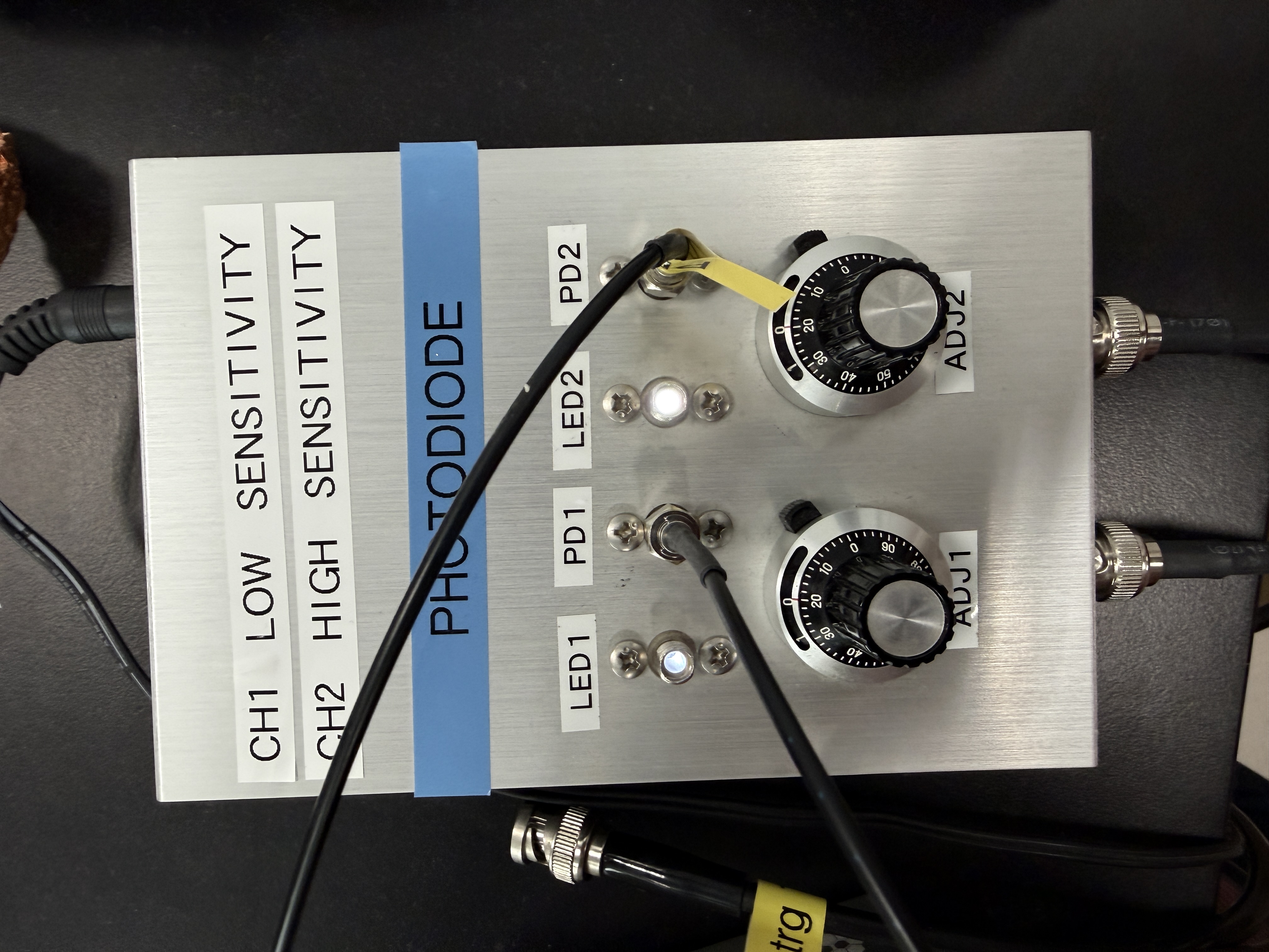
Photodiode box knob settings, recording 1 — Photodiode box, recording 1 (`sub-photodiode_01`). CH1 is LOW sensitivity (knob ADJ1), CH2 is HIGH sensitivity (knob ADJ2).

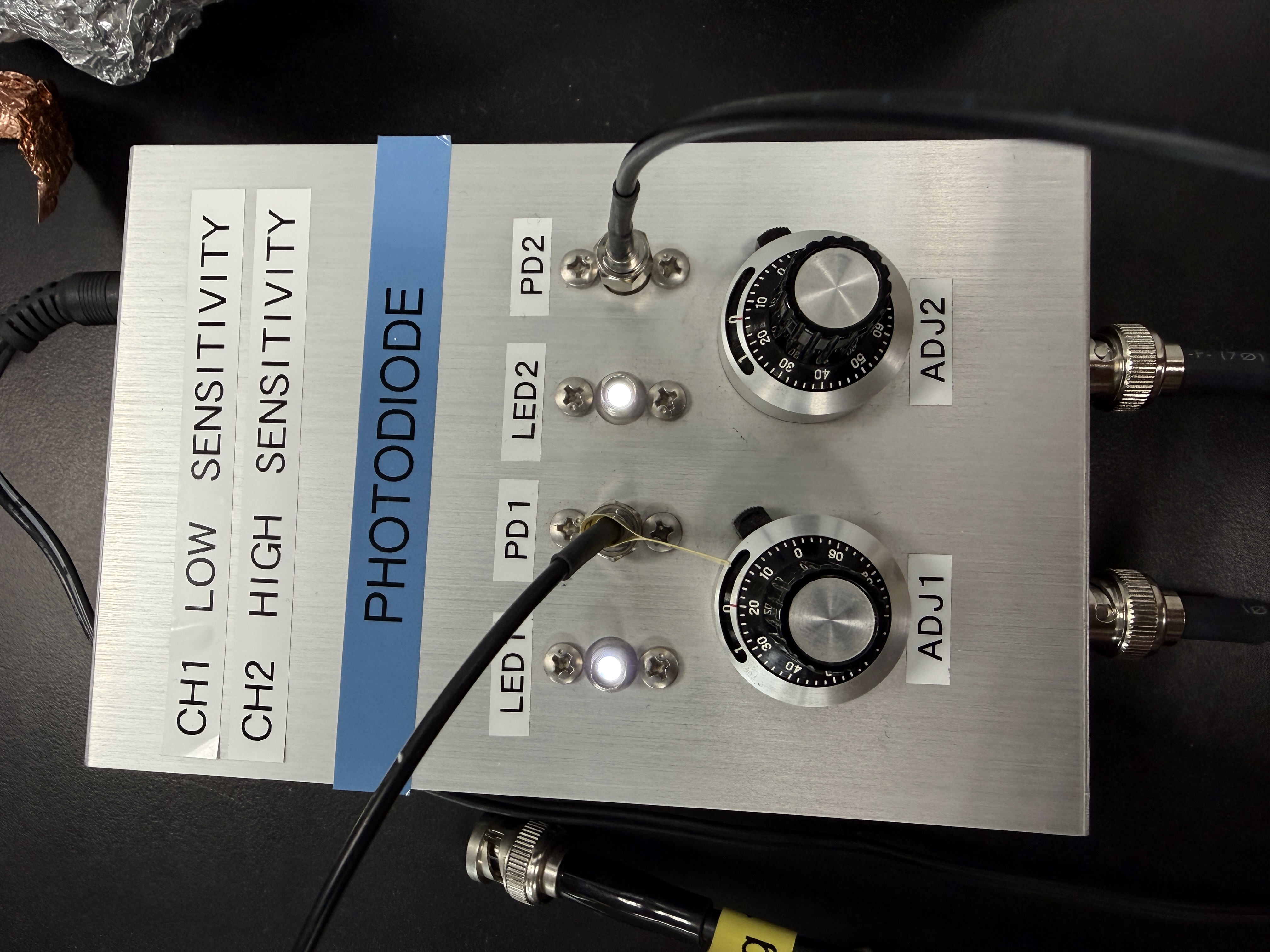
Photodiode box knob settings, recording 2 — Photodiode box, recording 2 (`sub-photodiode_02`). The LOW-sensitivity knob (ADJ1) is in the same position as recording 1, which is what makes the cross-recording comparison valid.

The two recordings 

Recording 1 - `sub-photodiode_01`
Box channel	Screen	MEG channel
CH1, LOW sensitivity	projector	233
CH2, HIGH sensitivity	stimulus computer	232
trigger (pixel mode)		224

Recording 2 - `sub-photodiode_02`
Box channel	Screen	MEG channel
CH1, LOW sensitivity	stimulus computer	233
CH2, HIGH sensitivity	projector	232
trigger (pixel mode)		224

Both recordings used 1000 trials. In recording 2 the high-sensitivity channel on the projector gave a noisier output that indexed the frame flip: multiple peaks within the 1 s white window rather than a boxcar, while the low-sensitivity channel on the stimulus computer was a smooth boxcar, 1 s on and 1 s off. That observation turns out to be the key to reading the data correctly (below).

Results 

Rising-edge lags from the clean low-sensitivity channel (projector in recording 1, stimulus monitor in recording 2), 1000 trials each:

Lag (rising edge)	Value	SD	n
Trigger 224 to stimulus monitor	+2.05 ms	0.21	1000
Trigger 224 to projector	+8.36 ms	0.48	1000
Stimulus monitor to projector	+6.31 ms		1000

Exactly 1000 trigger rising edges and 1001 screen rising edges were found in each recording, the extra one being the single-frame start flash. No data was lost. Both onsets are stable across the whole session (no drift) and jitter-free; the sub-millisecond SDs are 1 kHz sampling quantisation, not measured jitter. A constant correction is therefore exact.

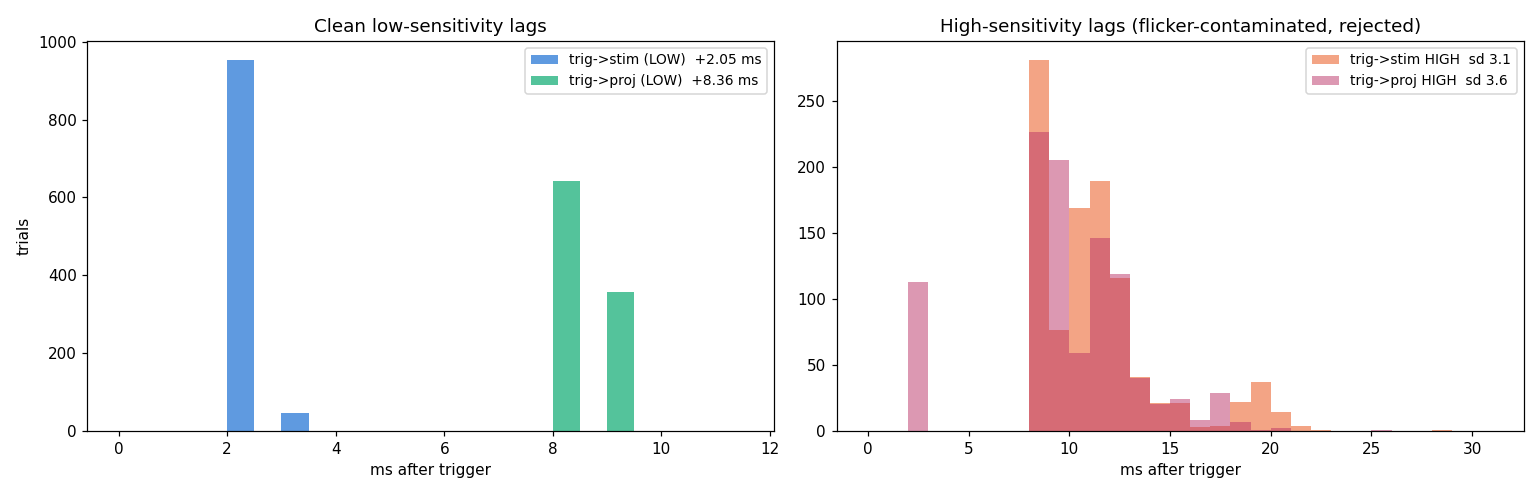
Lag distributions — Clean low-sensitivity lag distributions (left) and the flicker-contaminated high-sensitivity distributions (right), which are rejected (see below).

Use the low-sensitivity channel, not the average 

The original plan was to swap the channels and average the two measurements to cancel the sensitivity difference. The data show that averaging is the wrong move, and why.

The low-sensitivity channel gives clean, single-sample onsets for both screens. The high-sensitivity channel does not measure onset - it resolves sub-frame flicker: on the projector (a DLP) it becomes a dense train of ~1-4 ms pulses (~171 per 1 s block), and on the LCD it smears the onset across +8 to +28 ms. Proof it is an artefact: the same stimulus monitor, same trigger, reads +2.05 ms (sd 0.21) on the low-sensitivity channel but +10.86 ms (sd 3.07) on the high-sensitivity channel.

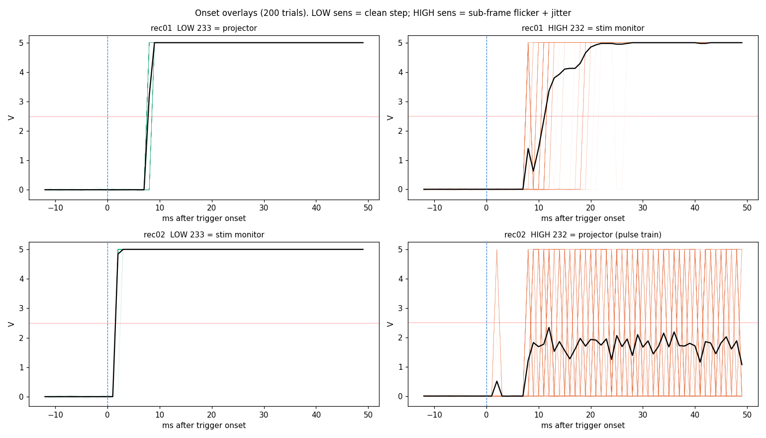
Onset overlays, low versus high sensitivity — 200 trials aligned to the trigger. The LOW-sensitivity channel is a clean single-sample step; the HIGH-sensitivity channel is smeared by sub-frame flicker and jitter.

The swap’s real value was giving the clean low-sensitivity channel a look at both screens (projector in recording 1, stimulus monitor in recording 2), which is an unbiased projector-versus-monitor comparison with no averaging. The counterbalance average would have given stimulus-to-projector +2.47 ms, wrong by about 3.8 ms purely because of the high-sensitivity artefact.

Verification 

The numbers were confirmed four independent ways: three Python detectors (50 percent threshold, sub-sample interpolation, derivative-peak) and an independent MATLAB / FieldTrip pipeline reading the raw .con files. All agree, and stimulus-to-projector = 6.31 ms in every method - it is independent of the trigger criterion because both onsets share the trigger reference.

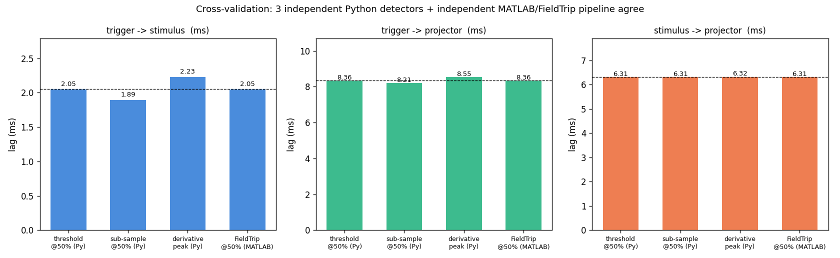
Four-method cross-validation — Four independent detectors / codebases agree on all three lags.

Why the lag exists 

The lag is hardware, not code.

The ~6 ms projector-minus-monitor gap is the PROPixx DLP pipeline latency: the projector buffers each frame and builds brightness by pulse-width-modulating micromirrors across the frame, which cannot start until the frame is received. A latency just under one frame (0.76 frame) is textbook DLP behaviour.
The ~2 ms trigger-to-monitor gap is the console monitor’s pixel response plus its input lag.

The trigger is emitted at the earliest deterministic point (frame scan-out via pixel mode), and the photodiode patch is at the top of the screen (scanned first), so no change to the PsychToolbox script reduces the true photon-arrival lag. The correct response is to measure it and correct for it.

Note

+8.36 ms is the correction for a stimulus at the top of the screen, where the patch sits. A stimulus lower on the screen is seen later by the raster scan time to that row (up to ~8 ms at the bottom). The ~6 ms projector term is common to all positions; the scan-position term is not. Place the photodiode patch at the height of the stimulus you care about, or record a projector photodiode live for per-trial correction.

What to do in your analysis 

Fallback: a constant, for data already acquired 

import mne
from apply_correction import correct_events, PROJECTOR_MS   # 8.36 ms

raw = mne.io.read_raw_kit("sub-XX_task.con", preload=True)
events = mne.find_events(raw, stim_channel="MISC 001")       # trigger 224
events = correct_events(events, raw.info["sfreq"], PROJECTOR_MS)  # shift +8.36 ms
epochs = mne.Epochs(raw, events, tmin=-0.2, tmax=0.8, baseline=(None, 0))

Use STIMULUS_MS (+2.05 ms) instead if the participant viewed the stimulus monitor rather than the projector.

Preferred: record a photodiode and correct per trial 

For real sessions, put a photodiode on the projector screen, patch it into an unused MISC channel, and add a small patch to a corner of your stimulus frame that changes with the event of interest. Then every trial carries its own ground truth and any future projector change cannot bias you.

from apply_correction import correct_events_photodiode

events = correct_events_photodiode(events, raw, "MISC 010")   # projector photodiode

Which analyses need it 

If your analysis…	Correction needed	Why
Compares conditions within one session	Optional	A common offset shifts all conditions equally and cancels in the contrast.
Reports absolute latencies (M100, P300)	Required	An uncorrected latency is 8.36 ms too early.
Compares against published latencies	Required	Other labs’ numbers are display-corrected; yours must be too.
Pools sessions recorded weeks apart	Recommended, per session	Verify the setup has not changed; record a live photodiode if unsure.
Uses stimulus offset as an event	Measure separately	Offset (white-to-black) was not characterised in this rise-only run and behaves differently from onset.
Needs better than about one frame absolute	Live photodiode	A constant cannot track a display change you did not measure.

Note

Correcting a common offset does not change the shape of an evoked response or the difference between two conditions in the same session. It changes reported latencies and cross-session or cross-lab comparisons.

Acquisition lessons 

These come from an earlier exploratory session (sub-photodiode-27-07-2026) whose photodiode channels were clipped. That session reported a higher, biased projector lag (~11.6 ms) and apparent projector width-drift and glitch frames; the clean, unclipped, counterbalanced re-acquisition above gives the stable +8.36 ms and did not reproduce onset instability. The lessons are why the re-acquisition was done and are worth following.

Set the input range so nothing clips. A clipped plateau collapses onto a handful of ADC codes, a 50 percent threshold is then not really 50 percent, and the bias cannot be removed afterwards. Check the plateau spans hundreds of ADC codes, not six.

Use DC coupling, not AC. DC passes the signal unaltered; AC inserts a series capacitor that high-pass filters at a few Hz, turning each 1 s plateau into a spike with an exponential decay whose tail re-crosses any fixed threshold (inflating the earlier event count from 1000 to 1326). Edge timing survives AC, but you lose the ability to verify the plateau.

Two channels fed the same frame must report the same pulse width. The single most useful sanity check. If they disagree they are triggering at different points on their luminance ramps, which biases their lags in opposite directions.

Counterbalance across recordings. Put the second photodiode on the other screen in each run, as done here, so the channel-sensitivity bias reverses and the clean channel measures both screens.

Keep both photodiodes at the same height on their screens. The raster draws top to bottom over 8.33 ms, so diodes at different heights read up to a full frame apart for reasons unrelated to display latency.

Other findings worth knowing 

The trigger line rises slowly and falls fast. Averaged over 1000 trials the rising edge fits an exponential RC curve with tau ~1.24 ms (R^2 0.96), while the falling edge completes inside one 1 ms sample - the signature of a passive pull-up with an active pull-down, almost certainly the opto-isolator on the MEG trigger input. Harmless if you threshold low on the curve, but “when the trigger fired” is ambiguous by 1-2 ms depending on criterion. Because every lag here uses the same trigger criterion, the stimulus-to-projector difference is unaffected.

Channel 229 is unused noise. It carries roughly 2 mV of crosstalk (0.08 percent of a logic level) plus one driven pulse per run from the start-flash block of the script; it is not a trial trigger and is ignored.

Use the PicoScope ``.mat`` export, not ``.psdata``. The .mat files load in one line with scipy.io.loadmat; there is no open Python reader for .psdata. The PicoScope also drops ~1 s between its sequential capture files, so those .mat files must not be concatenated as if continuous.

Code, data and pipelines 

Python pipeline: pipeline/mne_pipelines/photodiode_pipelines (rendered notebook: MNE)
MATLAB / FieldTrip pipeline: pipeline/field_trip_pipelines/photodiode (rendered notebook: FieldTrip)
Stimulus script: experiments/psychtoolbox/photodiode/photodiode_test.m
Definitive data: Box/MEG/Data/photo-diode (sub-photodiode_01.con, sub-photodiode_02.con). The earlier exploratory session is Box/MEG/Data/photo-diode/sub-photodiode-27-07-2026.

Note

Two comments in the stimulus script are out of date: it describes 500 ms phases where the loops actually produce 1 s, and it refers to channel 233 as the trigger reference where 233 is in fact the projector photodiode.